Inducing forced and auto-oscillations in one-dimensional photonic crystals with light

J. Eduardo Lugo; Rafael Doti; Noemi Sanchez; Jocelyn Faubert

doi:10.1117/1.JNP.8.083071

25 November 2014 Inducing forced and auto-oscillations in one-dimensional photonic crystals with light

J. Eduardo Lugo, Rafael Doti, Noemi Sanchez, Jocelyn Faubert

Author Affiliations +

Journal of Nanophotonics, Vol. 8, Issue 1, 083071 (November 2014). https://doi.org/10.1117/1.JNP.8.083071

Abstract

We induced forced and auto-oscillations in one-dimensional photonic crystals (1-D-PCs) with localized defects when light impinges transversally to the defect layer. The photonic structure used consists of a microcavity-like structure formed of two 1-D-PCs made of free-standing porous silicon, separated by a variable air gap (the defect) and the working wavelength is 633 nm. The force generation was made evident by driving a laser light by means of a chopper; the light hit the photonic structure and induced a vibration and the vibration was characterized by using a very sensitive vibrometer. For example, we measured peak displacements and velocities ranging from 2 to 167 μm and 0.4 to 2.1 mm/s with a power light level from 2.6 to 13 mW. In comparison, recent evidence showed that giant resonant light forces could induce average velocity values of 0.45 mm/s in microspheres embedded in water with a 43-mW light power.

1. Introduction

The concept of radiation pressure has been used in the past for manipulating micro-objects.¹ For example, optical tweezers are used to levitate viruses, bacteria, cells, and subcellular organisms.² Tweezing in free space with laser beams was established in the 1980s, but integrating the optical tweezers on a chip was a challenging task until recently. Reference 3 shows an alternative approach, where the shape of the optical trap can be tuned by the wavelength in coupled nanobeam cavities. Using these shapeable tweezers, the micromanipulation of polystyrene microspheres trapped on a silicon chip is achieved. On the other hand, the fast development of electromagnetic wave driven micro motors has motivated several research groups to investigate novel working principles for such micro motors,⁴ but there is a main obstacle. Normally, the radiation pressure is too small for these kinds of applications.⁵ Nonetheless, some resonance principles can be used to significantly increase the force, for instance, by using a waveguide made of lossless dielectric blocks, where the direction of the force exerted on the dielectric is parallel to the waveguide axis.⁶^,⁷ A second approach is with a Bragg waveguide based on a Fabry–Perot cavity in which the peak of the force only appears at the structures’ resonant frequencies and the force is normal to the waveguide wall.⁸ A third approach can use a one-dimensional photonic crystal (1-D-PC) with structural defects, where a localized mode results in strong electromagnetic fields around the position of the defect. Thus, the strong fields enhance the tangential and normal forces on a lossy dielectric layer.⁵

We can use this last approach to create a dynamical system capable of performing oscillations such as a forced oscillation, where an oscillation is imposed upon the system by and with the frequency of some external source (vibrator) of a sensibly different frequency, or auto-oscillations. The simplest auto-oscillating system⁹ consists of a constant source of energy, a regulatory mechanism that supplies energy to the oscillating system, and the oscillating system itself. There are two necessary features of auto-oscillations. The first is its feedback nature: on one hand, the regulatory mechanism controls the motion of the oscillating system but, on the other hand, it is the motion of the oscillating system that influences the operation of the regulatory mechanism. The second feature is a result of the fact that the loss of energy must be compensated by a constant source of energy. An example of a very simple oscillating system that can produce either auto or forced oscillations is a pendulum in a viscous frictional medium acted upon by a force of constant magnitude.

The present work is organized as follows: in the second section, we present the experimental details to fabricate the photonic structure and the bifoil. Then, we describe the setup to measure the structure movement for both the auto and forced oscillations. The third section describes the theory for inducing an electromagnetic force in the photonic structure with light. Also, a dynamical model for the mechanical auto and forced oscillations is presented. Next, we present and discuss the results where we compare the experimental results with theory. Finally, we wrap up the work with conclusions.

2. Experiment

2.1.

Methods and Materials

The 1-D-PCs were composed of alternating porous silicon (Psi) layers (Fig. 1) with refractive indices $n_{1} = 1.1$ , $n_{2} = 2$ , and layer thicknesses of $d_{1} = 326 \pm 11$ and $d_{2} = 435 \pm 11 nm$ . The refractive indices were chosen to work at the fourth photonic bandgap where localized states can be excited with the 633-nm red light. The fabrication details can be found elsewhere.¹⁰

Fig. 1

One-dimensional photonic crystal (1-D-PC) SEM picture showing the layers and a defect region (gap space between the two 1-D-PCs). The light impinges at the left interface (air) across the photonic structure and exits at the right interface on the substrate (glass).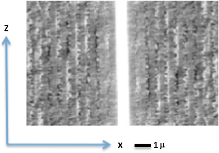

For building the vibrating device, two pieces of these samples have to be placed in a mirror-like symmetry, leaving a gap space between them. As the Psi foil is an elastic and very fragile material, it is difficult to manipulate because it is susceptible to presenting static electric charges. These characteristics, added to the poor mechanical resistance of the multilayer structure, impose the concept of building the simplest possible device. Another problem is that the Psi foil is not flat membrane because after being generated the multilayer porous structure is lifted from the c-Si. The resulting membrane accumulates mechanical stress that slightly deforms the original flat structure. Consequently, the gap space between foils is not homogeneous. Hence, we tried finding the right geometric condition in two configurations. In the first, we fixed two samples of Psi (one over the other) by means of the adhesive tape applied to one end of both specimens over a glass substrate. This is applied on both pieces placed together. In this case, the device has a cross section similar to a “V,” where the air gap is ideally linearly increased along the Psi foils as shown in Fig. 2. The second configuration consists of fixing each foil with the adhesive tape, but this time from opposite ends (double juxtaposed cantilever). Figure 3 shows the foils overlapped over the glass substrate. The experimental results confirmed that both configurations worked, but the second one was more effective and stable. Once we gained some experience in manipulating the foils along with mounting the device, we produced a dozen prototypes with small differences in piece shapes, and/or in the overlapped portion of Psi foils. The device showed a great robustness for all the prototypes tested.

Fig. 2

Schematic representation of the porous silicon bifoil device. In this case, the device presents single end Psi cantilevers.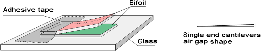

Fig. 3

Here, the foils are overlapped over the glass substrate but the cantilevers are juxtaposed from opposite ends.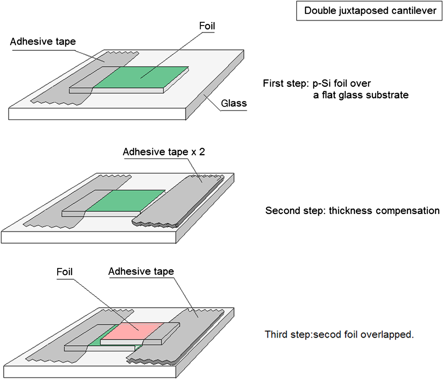

The general setup and layout are shown in Fig. 4 which consists of:

a. The Psi photonic structure device mounted on a glass substrate (bifoil device).
b. A precision rotation stage (DADEAL Inc.) with an X-Y micrometric positioning table (Parker).
c. A circular variable metallic neutral density filter (turning light attenuator). Newport model: 50G02AV.2, diameter 127 mm.
d. Infra-red bandpass filter (Techspec Edmund cut-off 650 nm)
e. He–Ne laser, power 13 mw, wavelength: 633 nm, beam diameter 2.58 mm (REO type LHRP 0501)
f. An electromagnetic beam chopper (MFE model R4077 open loop galvanometer 90 Hz)
g. A near-infrared (wavelength: 780 nm, power: 15 mw) laser vibration meter (VibroMet 500V)
h. A light detector (Tektronix Inc., model J6505, red candles)
i. A control computer
j. Oscilloscope (Agilent U 1604A, 40 MHz)
k. A signal generator (Topward Electric Instruments Ltd., model 8120)
l. A laser beam polarizer (Techspec Edmund 400 to 700 nm)

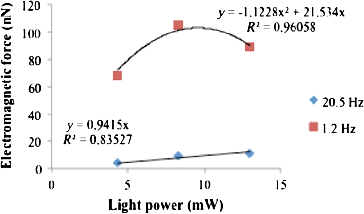
Fig. 4

Experimental setup for the oscillation measurements. (a) Auto-oscillation experimental configuration: (1) bifoil photodyne, (2) rotary and linear X-Y stages, (3) neutral filter wheel, (4) infrared bandpass filter, (5) He–Ne laser, (6) mechanical chopper, (7) vibrometer laser, (8) photocell, (9) computer, (10) oscilloscope, (11) vibrometer interface, (12) linear polarizer. The circuit shown represents a Schmitt trigger. (b) Forced oscillations experimental configuration: (1) bifoil photodyne, (2) rotary and linear X-Y stages, (3) neutral filter wheel, (4) infrared bandpass filter, (5) He–Ne laser, (6) mechanical chopper, (7) vibrometer laser, (8) photocell, (9) computer, (10) oscilloscope, (11) function generator, (12) linear polarizer. The insert image displays the main components of the real setup.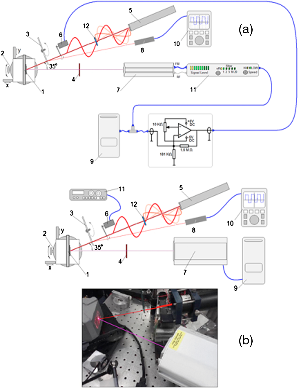

For the auto-oscillations, Fig. 4(a) shows the experimental setup where we introduced the bifoil device (1), which is mounted on rotary and X-Y linear stages (2), into a positive loop formed by the movement measuring the interferometer signal that is the real-time velocity signal provided by a very sensitive vibration meter (7,9,11) processed through an Schmitt trigger circuit, which controls the output of the pumping laser and chopper (5,6). This means that when the bifoil device starts moving, the circuit immediately blocks the laser light by means of the chopper. When the device returns to the initial position it triggers the pumping laser again and so on. Once the loop was closed, the device oscillated for a few seconds at different frequencies between 2 and 50 Hz. After that period, the device showed a clear stabilizing trend of auto-oscillations at 16.1 Hz with a duty cycle of 52%. At this frequency, the movement presented a purer spectrum with a narrow frequency spread and the device was stable for as long as 5 min. We used a Schmitt trigger circuit with an operational amplifier. By doing so, we have a wide range of parameters for circuit performance adjustments, and a high-speed loop reaction in reference to the mechanical deformation of the bifoil. The Schmitt trigger compares the velocity signal voltage of the vibration meter with a reference voltage. The resulting electric pulsed signal controlled the chopper. By means of the oscilloscope and a photocell [Fig. 4(a) components 8 and 10], we verified the signal and we could recognize the desired pulses of 1/25 of Voltage Direct VDC and the presence of a 60 Hz signal component (some millivolts induced from the power line). We did not filter this 60 Hz ‘‘noise’’ because it is useful to excite the loop as it helps to break the inertia. That is, it helps to initiate the device movement by adding a small vibration to the chopper blade that produces pumping light spikes. Otherwise, we excited the circuit by interrupting the pumping beam pass (manually) at a frequency of 2 to 3 Hz. This maneuver started the oscillation at that low frequency which was soon increased until reaching its stable oscillation mode of around 16.1 Hz.

For the forced oscillations, we used a similar setup but [Fig. 4(b)] the Schmitt trigger circuit was removed and it was replaced by a function generator (11) with an offset signal to control the duty cycle set at 75%. The rest of the experimental setup remained the same, including the laser light power, and we forced the bifoil to move at specific frequencies between 4 and 40 Hz, and found a very stable performance that lasted sometimes more than 20 h (until the samples showed physical damage).

In order to prevent undesirable reflection signals entering the vibration meter measures, we used an infrared bandpass filter (780 nm) and the option of playing with different power light intensities was considered as well the addition of a neutral wheel filter [Fig. 4(a), component 3]. The laser beam and the bifoil formed an angle of 35 deg in all the experiments. We tested the classic square waveform. As the chopper was based on a linear electromagnetic rotating transducer, the electric waveform used as excitation signals gave the corresponding light intensity shape in the time domain. We explored frequencies between 1 and 40 Hz. To ensure optimal blade movement alignment, we simply varied the DC level on the signal generator while looking for bigger signal amplitudes on the screen.

The photonic structure was tested and maintained at 23°C, and 30% relative humidity environmental conditions, as the Psi foil is hygroscopic. The surface area $A$ of this photonic device was $3 {mm}^{2}$ .

3. Theory

3.1.

Electromagnetic Force

Considering the structure depicted on Fig. 1, let us assume that light impinges on the off-axis direction at angle $θ_{0}$ with the electric field polarized in the $y$ -direction (TE polarization) and magnitude

Eq. (1)

E_{y} = E (x) e^{j (ω t - β z)},

where

Eq. (2)

E (x) = {\begin{cases} A_{0} e^{- j k_{0} (x - x_{0})} + B_{0} e^{j k_{0} (x - x_{0})} & x < x_{0} \\ A_{l} e^{- j k_{l} (x - x_{l})} + B_{0} e^{j k_{l} (x - x_{l})} & x_{l - 1} < x < x_{1} \\ A_{s} e^{- j k_{s} (x - x_{N})} + B_{s} e^{j k_{s} (x - x_{N})} & x_{N} < x \end{cases},

where all

A_{i}

’s and

B_{i}

’s are the complex amplitudes of the electric field in each region of the structure plus the air (0 label) and the substrate (s label) and the

k_{i}

’s are the wavevectors at different regions on the structure in the

x

-direction and

β

is the wavevector in the

z

-direction given by

ω n_{0} Sin (θ_{0}) / c

, where

n_{0}

and

θ_{0}

are the refractive index and angle of incidence on the air region,

c

is the speed of light in the vacuum, and

ω

is the light angular frequency. The

k_{i}

’s are given by

ω n_{i} Cos (θ_{i}) / c

, where

n_{i}

and

θ_{i}

are the refractive index and angle of incidence of region

i

, the latter given by

θ_{i} = Sin (n_{0} Sin (θ_{0}) / n_{i})

. By using a similar formalism as presented in Refs. 5 and 11, it is possible to show that for lossless dielectrics, the surface force density only exists in the

x

-direction and is given by

Eq. (3)

{〈 F_{x} 〉}_{T} = \sum_{l = 1}^{N} \frac{ε_{0}}{4} [{(\frac{n_{l - 1}}{n_{l}})}^{4} - 1] [\begin{array}{l} {| A_{l} |}^{2} + {| B_{l} |}^{2} + \\ 2 | A_{l} | | B_{l} | Cos (2 k_{l} d_{l} + φ_{A_{l}} - φ_{B_{l}}) \end{array}] + \frac{ε_{0}}{4} [{(\frac{n_{N}}{n_{s}})}^{4} - 1] [\begin{array}{l} {| A_{s} |}^{2} + | B_{s} |^{2} + \\ 2 | A_{s} | | B_{s} | Cos (φ_{A_{s}} - φ_{B_{s}}) \end{array}] + \sum_{l = 1}^{N} \frac{ε_{0}}{2} [{(n_{l})}^{2} - 1] | A_{l} | | B_{l} | [\begin{array}{l} Cos (φ_{A_{l}} - φ_{B_{l}}) - \\ Cos (2 k_{l} d_{l} + φ_{A_{l}} - φ_{B_{l}}) \end{array}],

where

ε_{0}

is the vacuum permittivity and

N

is the total number of layers. The complex amplitudes

A_{i}

’s,

B_{i}

’s and their phases

φ_{i}

can be calculated by using the well-known transfer matrix method¹² and their values depend on the light power.

3.2.

Mechanical Oscillations

An example of a very simple oscillating system that can produce either auto or forced oscillations is a pendulum in a viscous frictional medium acted upon by a force of constant magnitude. The differential equation of this dynamical system is

Eq. (4)

\begin{matrix} \ddot{x} + 2 h \dot{x} + ω_{0}^{2} x = {〈 a_{x} 〉}_{T} & j T < t < (n_{light} + j) T \\ \ddot{x} + 2 h \dot{x} + ω_{0}^{2} x = 0 & (n_{light} + j) T < t < (j + 1) T \\ j = 0, \dots m \end{matrix},

where

{〈 a_{x} 〉}_{T} = {〈 F_{x} 〉}_{T} A / m_{psi}

,

m_{psi}

, and

A

are the mass and the active surface area of the Psi bifoil,

h

is a damping coefficient,

ω_{0}

is the natural frequency of the system,

n_{light}

defines the duty cycle (fraction of the period where the light is on) which should take a value of 0.5 for the auto-oscillation case, and

j + 1

is the number of cycles that the light is on and off. The period

T

is related to the oscillator’s frequency

ω

as usual by

T = 2 π / ω

and is related to the natural frequency and damping coefficient as

ω^{2} = ω_{0}^{2} - h^{2}

. The self-oscillations arise, in principle, in the following manner. Considering the circuit of Fig. 4(a), there the energy is provided by a polarized laser light (5, 12) and a chopper (6). Initially, when the light is on, the electromagnetic force pushes down the bifoil (descending part). Now suppose that the energy dissipated throughout this part of the period is compensated by energy from the laser–chopper, since it is only then when the laser is in effective operation. If the compensation is exact in this part of the period, i.e., if there is neither a gain nor loss of energy, a prolonged oscillation will be reached. That is to say, the system will go into a steady oscillatory state with period

T

. In the second part of the period, the bifoil naturally goes into a damped oscillation until it stops and returns to the original position (ascending part). Mathematically, we can calculate this condition as

| 2 h \int_{0}^{T / 2} {\dot{x}}^{2} d t | = | \int_{0}^{T / 2} {〈 a_{x} 〉}_{T} \dot{x} d t | = | \int_{0}^{T / 2} {〈 a_{x} 〉}_{T} d x |

for

t \in [0, T / 2]

, we can approximate this condition, without knowing the exact solution of Eq. (4), by using the maximum values for the displacement

x_{p}

and velocity

V_{p}

. Therefore, the auto-oscillation condition reads:

Eq. (5)

| 2 h V_{p}^{2} T / 2 | = | {〈 a_{x} 〉}_{T} x_{p} | .

4. Results

4.1.

Electromagnetic Force

Now let us use Eq. (3) to calculate the electromagnetic force induced in the structure. We know that the force is going to depend on the defect length, the light power level, and the angle of incidence. For instance, in Fig. 5, we can observe the force profiles for different gap lengths and light powers at normal incidence. Clearly, under these conditions there is a resonance at a defect length of $7 x (n_{1} d_{1} + n_{2} d_{2})$ for all light powers. For 13 mW, the lowest force magnitude is found at $10 x (n_{1} d_{1} + n_{2} d_{2})$ with a value of approximately 10 nN. Moreover, if we plot the electromagnetic force at resonance against light power (Fig. 6), the relationship is linear with a slope of $19.7 nN / mW$ .

Fig. 5

Electromagnetic force profiles for different optical power levels and defect lengths. The light impinges with an angle of zero degrees and TE polarization.

Fig. 6

Theoretical linear relationship between the electromagnetic force and light power.

Now, if we use an angle of incidence of 35 deg, we observe that the electromagnetic force density [Eq. (3)] oscillates between the values of 3.5 and $2 mN / m^{2}$ for defect lengths ranging from 10 nm up to more than 1 mm (Fig. 7). Without a doubt there is no resonance state under these conditions and on average we expect a force density of the order of $2.75 mN / m^{2}$ , which gives a force of the order of 8.25 nN ( $3 \times 10^{- 6} m^{2} \times 2.75 mN / m^{2}$ ) for a wide range of gap lengths.

Fig. 7

Theoretical surface force density [Eq. (3)] at different gap lengths. The surface density force oscillates between 2 and $3.5 mN / m 2$ with gap lengths of more than 1 mm for an angle of incidence of 35 degrees.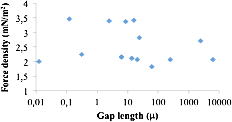

4.2.

Auto-Oscillations

In Fig. 8(a), we observe the experimental bifoil velocity time series, where we can see an asymmetry between the descending (positive voltage) and the ascending (negative voltage) parts, implying that the damping coefficient of the descending part is higher than the coefficient of the ascending part. Figure 8(b) shows the power spectral density (PSD) of the velocity time series and only one peak appears at 16.1 Hz. We found experimental values for $x_{p} = 4.12028 μ m$ and $V_{p} = 0.42 mm / s$ . We can estimate the parameter ${〈 a_{x} 〉}_{T}$ as follows: the surface area $A$ of this photonic device was $3 {mm}^{2}$ and the total thickness is $20 x (761 \times 10^{- 9}) m^{2}$ , which gives a volume of $4.566 \times 10^{- 11} m^{3}$ . The volumetric density of each layer is the product of $(1 - P) x 2330 kg / m^{3}$ , where $P$ means porosity. The value of $2330 kg / m^{3}$ corresponds to the volumetric density of c-Si. Since each foil is a multilayer structure that contains two different porosities, there are two different volumetric densities. In order to obtain an effective volumetric density, we can take a weight average of both densities where the weights correspond to each thickness. The final result is $586 kg / m^{3}$ . Multiplying the volume times, the effective volumetric density gives us the mass estimation, which has a value of $2.676 \times 10^{- 8} Kg$ . As before, we used the average value for the force density ${〈 F_{x} 〉}_{T}$ that equals $2.750 \times 10^{- 3} N / m^{2}$ given that $A = 3 \times 10^{- 6} m^{2}$ and the value of ${〈 a_{x} 〉}_{T}$ is $0.308 m / s$ . According to the values obtained for $x_{p}$ , $V_{p}$ , $T$ , and ${〈 a_{x} 〉}_{T}$ , we found that the auto-oscillation condition [Eq. (5)] gives a value for $h$ of 115.95.

Fig. 8

Auto-oscillation experimental and theoretical results. (a) Experimental velocity time series, (b) experimental power spectral density for the velocity, (c) theoretical velocity time series, (d) theoretical power spectral density for the velocity, (e) theoretical displacement time series (insert).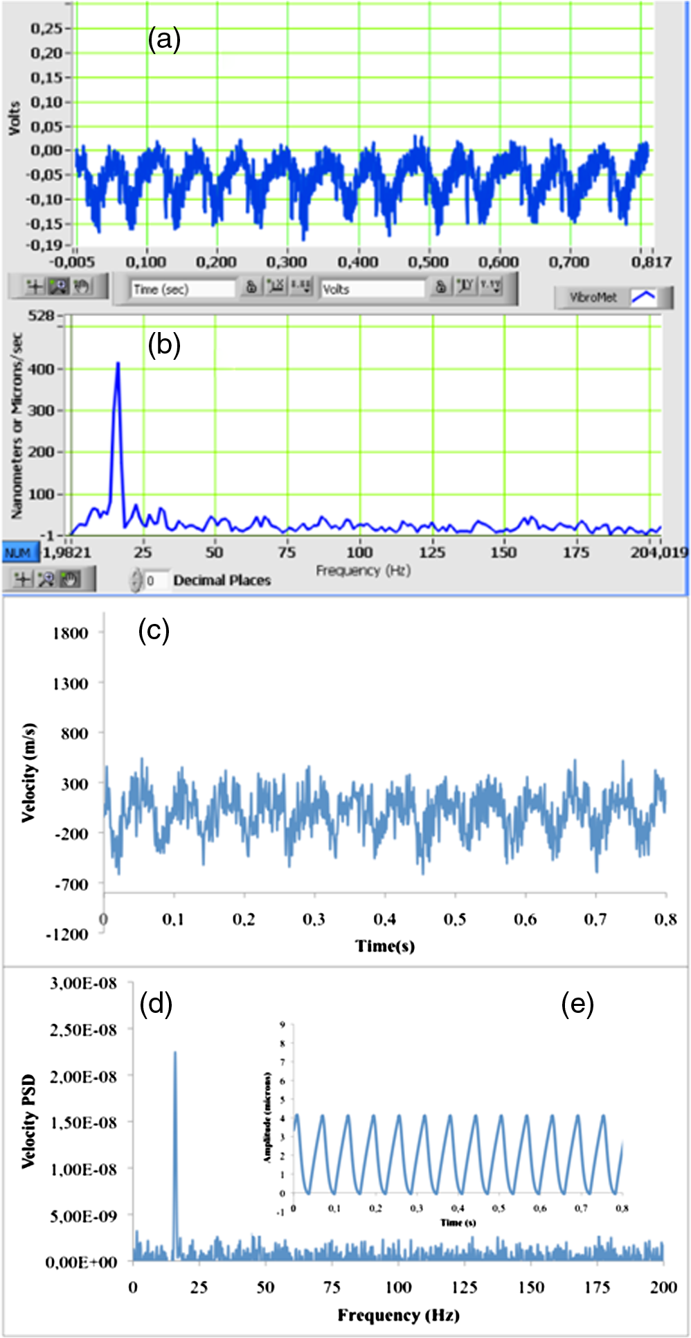

We simulated Eq. (4) by using MATLAB® and the best fit we found uses the aforementioned parameters; only the parameter $h$ needed to be multiplied by 16.4 instead of 2 in the descending part and we use the experimental value $n_{light} = 0.52$ . Figures 8(c) and 8(d) show the simulated velocity time series and its PSD, which fit nicely with the experimental measurements. In order to take uncontrollable vibration effects into account, 60 Hz noise, etc., we added a zero-mean random noise to the simulated velocity time series. The amplitude of this noise signal was 25% of the peak velocity amplitude. Figure 8(e) shows the simulated displacement time series with a maximum value of $4.119 μ m$ .

4.3.

Forced Oscillations

First, we simulated Eq. (4) by using MATLAB and kept the same parameter values for $h$ , $ω_{0}$ , ${〈 a_{x} 〉}_{T}$ as in the auto-oscillations case. We used a value for $n_{light}$ of 0.75. The parameter $T$ was changed according to the experimental forced frequency (8.6 Hz). Second, we compared the simulation and the experimental results as shown in Figs. 9(a) and 9(b) for a driven frequency of 9 Hz. It is known that the bifoil vibrates mainly at 8.6 Hz, but the appearance of high harmonics is evident. The maximum displacement was 8.176. The theoretical results are observed in Figs. 9(c) to 9(e). Again, the fit is very good and we were able to reproduce the first three harmonics and a maximum displacement of $8.540 μ m$ .

Fig. 9

Forced-oscillation experimental and theoretical results. (a) Experimental velocity time series, (b) experimental power spectral density for the velocity, (c) theoretical velocity time series, (d) theoretical power spectral density for the velocity, (e) theoretical displacement time series (inset).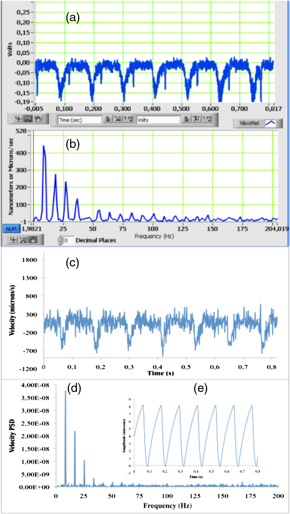

Third, we improved the characterization of the forced oscillations by measuring the displacement amplitude versus forced frequency or light power levels. Figure 10 shows a typical vibration measurement output. The optical pumping signal had a square waveform shape with a duty cycle of approximately 75%, a frequency of 5 Hz, and a power of 13 mW. In Fig. 10, we can observe that the photonic structure oscillates mainly at a frequency of 4.9 Hz with an amplitude of approximately $17 μ m$ and an acceleration of $0.02 m / s^{2}$ .

Fig. 10

A typical vibration measurement, where we can see the amplitude of the movement, the velocity, the acceleration, and the velocity Fourier spectrum.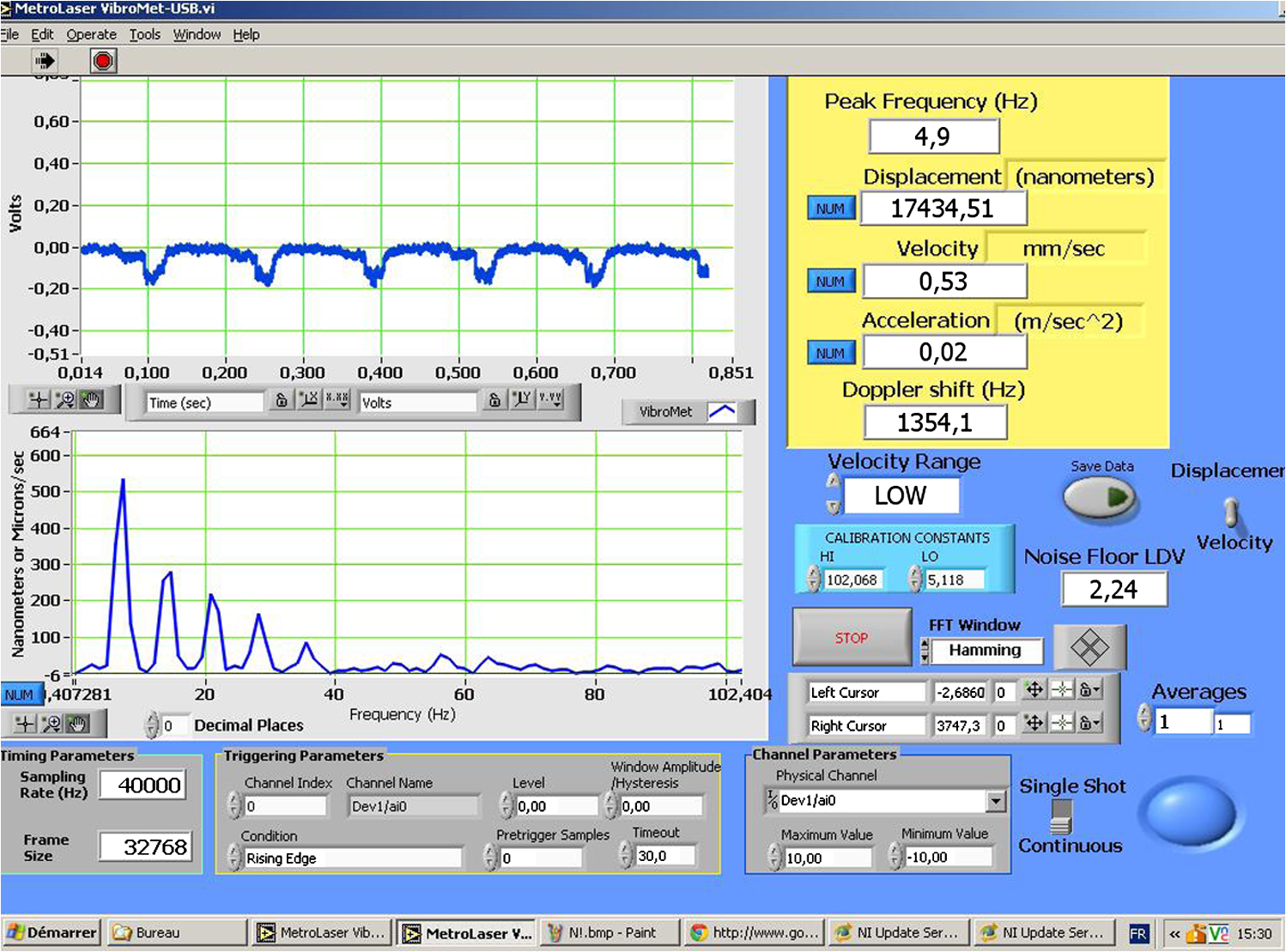

Figure 11 shows how the bifoil displacement decreases when the forced frequency increases approximately following an $L / ν^{n}$ relationship with an exponent $n = - 1.812$ and a constant $L = 133.6$ ${Hz}^{- 1.812} μ m$ . Again, we kept the same parameter values for $h$ , $ω_{0}$ and $n_{light}$ and only changed $T$ . The parameter ${〈 a_{x} 〉}_{T}$ is adjustable and serves to estimate the electromagnetic force.

Fig. 11

The bifoil photodyne displacement behavior with different forced frequencies at a light power level of 13 mW.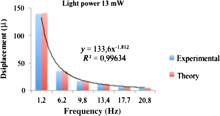

Equation (4) fits the bifoil displacement as shown in Figs. 11 and 12 very well under different experimental conditions. In Fig. 12, we observe that the bifoil displacement increases as the power light increases when the forced frequency is fixed.

Fig. 12

The bifoil photodyne displacement behavior with light power at a forced frequency of 20.5 Hz.

Figure 13 shows the bifoil photodyne displacement behavior when the light power increases. When the forced frequency is high (20.5 Hz) the relationship may be linear, while at low frequencies it is not. It seems that at low frequencies, the structure may be closer to the resonance condition for a certain surface area. Note that this surface area is not the whole available surface area of the bifoil and it could be different from one cycle to another. In Fig. 14, we observe as in Fig. 11 that the bifoil displacement decreases when the forced frequency increases for two different light power levels.

Fig. 13

The bifoil photodyne displacement behavior with light power and two different forced frequencies.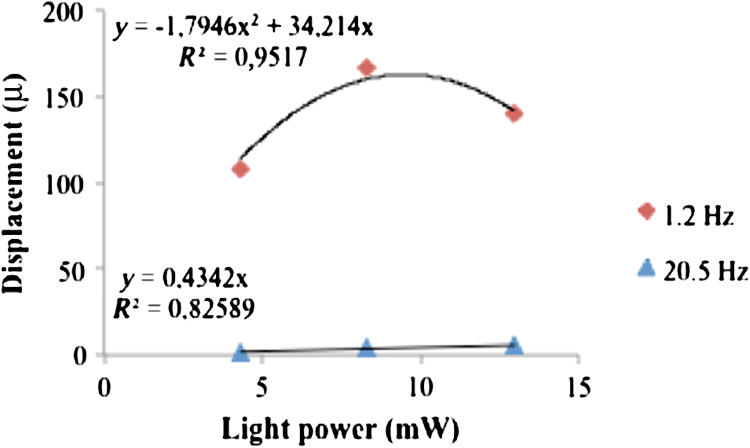

Fig. 14

The bifoil photodyne displacement behavior with the forced frequency at two different light power levels.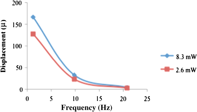

Since the parameter ${〈 a_{x} 〉}_{T}$ is given by ${〈 F_{x} 〉}_{T} A / m_{psi}$ , by knowing the bifoil mass $m_{psi}$ , it is possible to know the electromagnetic force ${〈 F_{x} 〉}_{T} A$ . In Fig. 15, we observe that the relationship between the electromagnetic force of the light power may be linear for high frequencies, but not for low frequencies. Theoretically, a linear relation should be expected as shown before in Fig. 6. It seems that at low frequencies, the bifoil structure is closer to the resonance condition for a certain surface area but since we are not controlling the gap length, the resultant electromagnetic force does not follow a simple relationship but depends on how the final distribution of the gap length is from one cycle to another. We think the bifoil structure is close to resonance because the order of magnitude for the electromagnetic force values is similar to the theoretical values shown in Fig. 5.

Fig. 15

The induced electromagnetic force behavior with light power at two different forced frequencies.

5. Conclusions

In conclusion, we were able to use light to induce forced and auto-oscillations in a photonic crystal structure. For forced oscillations, the highest bifoil displacements were found at low frequencies. At high frequencies, the displacements increase when light power increases. At low frequencies, we found the highest electromagnetic force values whose order of magnitude is comparable with theoretical values predicted close to resonance. The structure was shown to be very stable for several hours when the light pumping was controlled by the function generator.

In the auto-oscillation case, we only found a frequency of 16.1 Hz and its stability lasted a few minutes. This is because the conditions (active bifoil area, elastic recovery forces, irregular PSi pieces surface, etc.) are more critical for the closed loop operation (auto-oscillator) implementing the loop via a Schmitt trigger. In the open loop operation type, we found several movement modes where amplitudes reduced at higher frequencies according to a nonlinear attenuation along the frequency interval limited to 100 Hz. In the closed loop (auto-oscillator) operation type, the displacement mode presented a narrow spectrum centered at the main oscillation frequency.

Finally, our findings suggest the possibility of using this electromagnetic force to create new devices that can be activated only with light.

Acknowledgments

This work was supported by an NSERC Discovery operating grant. J. E. Lugo would like to thank Dr. M. Beatriz de la Mora and Dr. J. Antonio del Rio for the photonic crystal fabrication. R. Doti, J. E. Lugo, and N. Sanchez performed all the experiments. J. E. Lugo and R. Doti performed all the data analysis. J. Faubert, contributed with reagents, materials and analysis tools. J. E. L., R. D., J. F. wrote the manuscript. All authors reviewed the manuscript. This submission is based upon a presentation that J. E. Lugo is making.

References

1.

K. DholakiaG. SpaldingM. MacDonald, “Optical tweezers: the next generation,” Phys. World, 15 (10), 31 –35 (2002). PHWOEW 0953-8585 Google Scholar

2.

A. AshkinJ. M. Dziedzic, “Optical trapping and manipulation of viruses and bacteria,” Science, 235 (4795), 1517 –1520 (1987). http://dx.doi.org/10.1126/science.3547653 SCIEAS 0036-8075 Google Scholar

3.

C. Renautet al., “On chip shapeable optical tweezers,” Sci. Rep., 3 2290 (2013). http://dx.doi.org/10.1038/srep02290 SRCEC3 2045-2322 Google Scholar

4.

E. Higurashiet al., “Optically induced rotation of dissymmetrically shaped fluorinated polyimide micro-objects in optical traps,” J. Appl. Phys., 82 (6), 2773 –2779 (1997). http://dx.doi.org/10.1063/1.366163 JAPIAU 0021-8979 Google Scholar

5.

J. M. LiG. J. Shan, “Enhancement of electromagnetic force by localized fields in one-dimensional photonic crystal,” Prog. Electromagn. Res., 10 59 –70 (2009). http://dx.doi.org/10.2528/PIERM09102202 PELREX 1043-626X Google Scholar

6.

R. Gomez-Medinaet al., “Resonant radiation pressure on neutral particles in a waveguide,” Phys. Rev. Lett., 86 (19), 4275 –4277 (2001). http://dx.doi.org/10.1103/PhysRevLett.86.4275 PRLTAO 0031-9007 Google Scholar

7.

A. Mizrahi, “Torque and longitudinal force exerted by eigenmodes on circular waveguides,” Phys. Rev. A, 78 023802 (2008). http://dx.doi.org/10.1103/PhysRevA.78.023802 PLRAAN 1050-2947 Google Scholar

8.

M. L. Povinelliet al., “Slow-light enhancement of radiation pressure in an omnidirectional-reflector waveguide,” Appl. Phys. Lett., 85 1466 (2004). http://dx.doi.org/10.1063/1.1786660 APPLAB 0003-6951 Google Scholar

9.

J. E. Lugoet al., “The bifoil photodyne: a photonic crystal oscillator,” Sci. Rep., 4 3705 (2014). http://dx.doi.org/10.1038/srep03705 SRCEC3 2045-2322 Google Scholar

10.

R. Navaet al., “Refractive index contrast in porous silicon multilayers,” Phys. Status Solidi C, 6 1721 (2009). http://dx.doi.org/10.1002/pssc.v6:7 PSSCGL 1610-1634 Google Scholar

11.

A. MizrahiL. Schachter, “Electromagnetic forces on the dielectric layers of the planar optical Bragg acceleration structure,” Phys. Rev. E, 74 036504 (2006). http://dx.doi.org/10.1103/PhysRevE.74.036504 PLEEE8 1063-651X Google Scholar

12.

Y. Pochi, Optical Waves in Layered Media, 102 –141 John Wiley & Sons, Inc., New York (1988). Google Scholar

Biography

J. Eduardo Lugo received his PhD degree in physics from Morelos State University, Mexico. He was a professor at Morelos State University and the National Autonomous University of Mexico (UNAM). He was a postdoctoral fellow at University of Rochester and McGill University. Currently, he is at the Visual Psychophysics and Perception Laboratory, working with different photonic applications ranging from photonic crystals and near-infrared spectroscopy of the brain. He is a member of SPIE.

Rafael Doti is an electronic and mechanical engineer from the engineering faculty of Buenos Aires University (FIUBA), Argentina. He was a researcher at the FIUBA Laser Laboratory and he taught physics at the Physics Department (FIUBA). He joined the Visual Psychophysics and Perception Laboratory at Montreal University, where he has helped develop new methods, experiments, and devices for sensory stimulation and data record, Shack–Hartmann wave front analysis, and near-IR brain spectroscopy.

Noemi Sanchez working on one-dimensional (1-D) photonic structures. She received her BA degree in applied physics from the Autonomous University of Puebla (BUAP), México, in 2011. Subsequently, she received her master’s degree from the National Institute of Astrophysics, Optics and Electronics in 2013. Her thesis included a research stay at the University of Montreal to experimentally work with porous silicon nanostructures. Currently, she is pursuing her PhD in applied physics at the BUAP. She is a member of OSA and SPIE

Jocelyn Faubert received his PhD degree in psychophysics from Concordia University. He then started a postdoctoral fellowship at Harvard University. He is full professor at University of Montreal at the School of Optometry. He is the director of the Visual Psychophysics and Perception Laboratory. He is a senior chair holder for the Natural Sciences and Engineering Research Council-Essilor Industrial Research Chair. He was founder of Ophtalox, Inc., CogniSens, Inc., and CogniSens Athletics, Inc. Companies.

CC BY: © The Authors. Published by SPIE under a Creative Commons Attribution 4.0 Unported License. Distribution or reproduction of this work in whole or in part requires full attribution of the original publication, including its DOI.

Citation Download Citation

J. Eduardo Lugo, Rafael Doti, Noemi Sanchez, and Jocelyn Faubert "Inducing forced and auto-oscillations in one-dimensional photonic crystals with light," Journal of Nanophotonics 8(1), 083071 (25 November 2014). https://doi.org/10.1117/1.JNP.8.083071

Published: 25 November 2014

Access the abstract

JOURNAL ARTICLE
13 PAGES

DOWNLOAD PAPER SAVE TO MY LIBRARY

GET CITATION

CITATIONS

Cited by 6 scholarly publications.

Explore citations on Lens.org

KEYWORDS

Photonic crystals

Electromagnetism

Bandpass filters

Silicon

Glasses

Control systems

Dielectrics

1.

Introduction

2.

Experiment

2.1.

Methods and Materials

Fig. 1

Fig. 2

Fig. 3

Fig. 4

3.

Theory

3.1.

Electromagnetic Force

Eq. (1)

Eq. (2)

Eq. (3)

3.2.

Mechanical Oscillations

Eq. (4)

Eq. (5)

4.

Results

4.1.

Electromagnetic Force

Fig. 5

Fig. 6

Fig. 7

4.2.

Auto-Oscillations

Fig. 8

4.3.

Forced Oscillations

Fig. 9

Fig. 10

Fig. 11

Fig. 12

Fig. 13

Fig. 14

Fig. 15

5.

Conclusions

Acknowledgments

References

Biography

Show All Keywords

Keywords/Phrases

Search In:

Publication Years